Exploring fbprophet with stock scrips
Fbprophet is a time-series forecasting package open-sourced by Facebook in 2017. This is an additive model which provides intuitive input parameters, allowing users with domain knowledge to tweak it with very little statistical knowledge of the internals. Part of the intuitiveness stems because it allows users to specify holidays and changepoints and also use user-added seasonality as input. In this blog post, we are going to exchange some ideas on how to use the package better.
For training data, we are going to use a stock symbol data traded on the National Stock Exchange (NSE) of India. To ease our access to data, we will be downloading the historical data from Yahoo Finance. It downloads as a CSV file which we can open with Pandas for further examination.
import pandas as pd
from fbprophet import Prophet
from fbprophet.plot import add_changepoints_to_plot
from matplotlib import pyplot as plt
import holidays
import warnings
warnings.simplefilter('ignore')
data = pd.read_csv("TATAMOTORS.BO.csv", parse_dates=['Date'])
data.head()
| Date | Open | High | Low | Close | Adj Close | Volume | |
|---|---|---|---|---|---|---|---|
| 0 | 1991-01-02 | 20.9601 | 21.8584 | 20.9601 | 21.8584 | 4.024777 | 0.0 |
| 1 | 1991-01-03 | 20.9601 | 21.8584 | 20.9601 | 21.8584 | 4.024777 | 0.0 |
| 2 | 1991-01-04 | NaN | NaN | NaN | NaN | NaN | NaN |
| 3 | 1991-01-07 | 20.3613 | 21.2596 | 20.0618 | 21.1098 | 3.886938 | 0.0 |
| 4 | 1991-01-08 | NaN | NaN | NaN | NaN | NaN | NaN |
Further examination shows us that we have 28 years of daily OHLC (open, high, low, close) data. That’s a lot of data. For our modelling efforts, we will use the closing price of the day (in the Close column). First off, let’s visualise the stock’s movements over the years.
_ = data.set_index('Date')['Close'].plot()
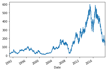
Part of the reason for this stock’s meteoric spike was its purchase of Jaguar & Land Rover brands (JLR) in July 2008. For our purpose, we will use a 5 year period to train and produce a forecast for the upcoming 6 months starting from the last date in the training data. This reduced time window 0f 5 years (than 14 years) will allow us to capture movements in price after the acquisition more closely.
df = data.tail(2000).set_index('Date')['Close']
df = df.reset_index().rename(columns={'Date': 'ds', 'Close': 'y'})
_ = df.set_index('ds')['y'].plot(figsize=(12, 7))

holidays = df[df.y.isnull()]
holidays = holidays.rename(columns={'y': 'holiday'}).fillna('Other')
holidays.loc[:, 'ds'] = holidays['ds'].dt.strftime('%Y-%m-%d')
# holidays = pd.concat([holidays, pd.read_csv("/Users/fibinse/Downloads/holidays.csv")])
holidays.loc[:, 'upper_window'] = 1
holidays.loc[:, 'lower_window'] = 0

print(df.shape)
df = df.dropna()
df.shape
(2000, 2)


(1994, 2)
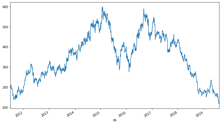
The fbprophet model interface is similar to the one provided by sklearn. Before that, we will split the time series that we visualised above into a training and testing set.
N = int(df.shape[0] * .78)
train, test = df.iloc[300 :N], df.loc[N: N+200]
test.loc[:, 'ds'] = pd.to_datetime(test.ds)
print(train.ds.describe(), '\n\n\n', test.ds.describe())
count                    1255
unique                   1255
top       2016-09-08 00:00:00
freq                        1
first     2012-09-20 00:00:00
last      2017-10-30 00:00:00
Name: ds, dtype: object


 count                     201
unique                    201
top       2017-10-30 00:00:00
freq                        1
first     2017-10-23 00:00:00
last      2018-08-08 00:00:00
Name: ds, dtype: object
We have split the data into a training set with 1255 days of data and test set with 200 days of data. Now, we instantiate a model and fit it on the training data.
model = Prophet()
_ = model.fit(train)
INFO:fbprophet:Disabling daily seasonality. Run prophet with daily_seasonality=True to override this.
We will now use fbprophet’s make_future_dataframe function to create a dataframe of future dates, with the same dimension as that of the test dataframe. The include_history makes sure that we strictly get only future dates from the end of the training data set.
future = model.make_future_dataframe(periods=test.shape[0], include_history=False)
future = model.predict(future)
The predict method creates a rich future dataframe where each date is assigned a prediction (yhat) along with its uncertainty intervals.
_ = model.plot(future)
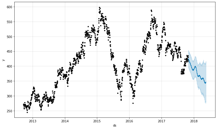
We will use the mean absolute error function to calculate the error in our forecast.
def mean_absolute_error(y_true, y_pred):
    y_true, y_pred = pd.np.array(y_true), pd.np.array(y_pred)
    return round(pd.np.mean(pd.np.abs((y_true - y_pred))), 1)
print("MAE in baseline forecast: INR {:.1f}".format(mean_absolute_error(test['y'], future['yhat'])))
MAE in baseline forecast: INR 37.3
When we initialise a Prophet model, we have a handful of features which we could tune to improve our forecast.
-
growth='linear'| 'logistic': Since the stock symbol as financial instrument does not really have an upper limit to its value, we will use Prophet’s linear model. If you were to forecast things which can have a saturating growth, like computing capacity in a server or human population in a given area, we could go with the logistic model. -
Changepoints: Prophet accomodates a list of dates as input if we wanted it to keep it from calculating them instead. These dates can be passed via thechangepointsattribute. If this attribute is not provided, it then picksn_changepointsfrom the firstchangepoint_rangerange of the data. For example, default values for these are:n_changepoints=25&changepoint_range=0.8, this means that we are asking the model to uniformly sample 25 points from the first 80% of the training data. These should be used to indicate abrupt changes in the behaviour of the time series. In case of stock symbols, it may be a good idea to include the dates at which quarterly results were announced. -
changepoint_prior_scale: controls the model’s flexibility to including changepoints. In my experience,changepoint_prior_scalehas been more useful than specifyingchangepointsdates or specifying thechangepoint_range. -
yearly_seasonality,weekly_seasonalityanddaily_seasonalityattributes control the seasonality that the model should capture. The model captures these seasonalities as additive components in the forecast, which sometimes helps in observing if the model has captured the data correctly. I usually turns these off and add seasonal regressors using theadd_seasonalityfeature. -
We can control how the
holidaysaffect our model by passing a columnprior_scalealong a dataframe of dates and holiday names. This dataframe can additionally include the range of days around the holiday date as part of the holiday. A row for the Christmas holiday week, could haveupper_window=7andlower_window=0which will then include 25th Dec to 2nd Jan as holidays. If we don’t want to specify dates, we could useholidays_prior_scaleparameter to control the strength of the holiday component in the model. Its default value is 10.0. -
The
seasonality_modeparameter which defaults to'additive'means that components are added to the trend. From the official documentation, when “the seasonality is not a constant additive factor as assumed by Prophet, rather it grows with the trend. This is multiplicative seasonality.” and that is when we should set theseasonality_mode=multiplicative.seasonality_prior_scale: Larger values allow the model to fit larger seasonal fluctuations, smaller values dampen the seasonality. Can be specified for individual seasonalities using add_seasonality.” -
interval_widthsets the width of the confidence interval around the forecast.
We have gone ahead and disabled all seasonality parameters which appear by default in the model. Additionally, we have increased the changepoint_prior_scale by a small amount (0.02).
model = Prophet(
                daily_seasonality=False,
                weekly_seasonality=False,
                yearly_seasonality=False,
                changepoint_prior_scale=0.07,
                )
# add yearly seasonality
model.add_seasonality('yearly', period=365.25, fourier_order=10)
_ = model.fit(train)

future = model.make_future_dataframe(periods=test.shape[0], include_history=False)
future = model.predict(future)

# join the actual value with the forecast
_ = data.merge(future[['ds', 'yhat']],
           left_on='Date', right_on='ds',
           how='left'
           ).set_index('Date')[['Close', 'yhat']].dropna()

# calculate the mean absolute error
mae_error = mean_absolute_error(_['yhat'], _['Close'])
print("Mean absolute error: ", round(mae_error, 1))
_ = _.plot(title='Prediction vs Actual')
Mean absolute error: 17.0
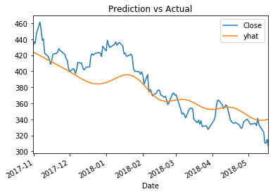
There is quite a bit of work to be done to improve the forecast as the plotted components tell us below.
_ = model.plot_components(future)
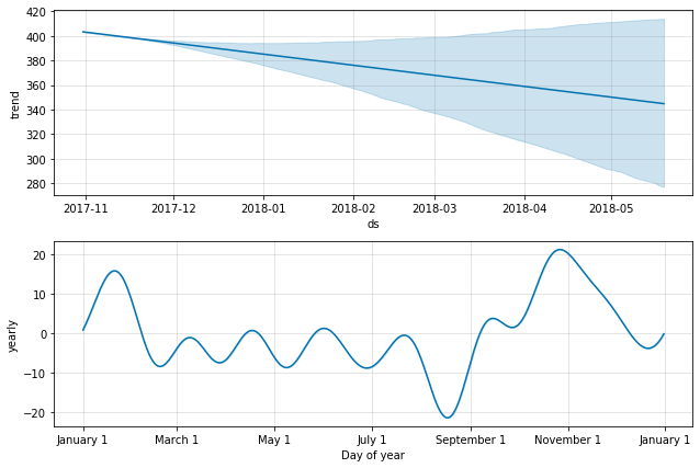
The trend-plot in the first diagram shows an increasingly spreading confidence interval. Beyond a month of forecast, the trend cannot be really trusted. The yearly component also shows the forecasted nature of the stock symbol: it spikes by 15% at the beginning of the year, hits a trough near September where it falls by a bit more than 20% and tries to recover again in November. Do remember, this is again only the forecasted components.
Once the data has been fitted, we can use add_changepoints_to_plot to plot the dates as red-dotted lines for visual inspection.
fig, axes = plt.subplots(1, 1, figsize=(8, 5))

# plot forecast with the actual values
axes.set_title('Observed changepoints. MAE : {:,.0f}'.format(round(mae_error)))
_ = model.plot(future, ax=axes)

# plot change points that the model has observed
a = add_changepoints_to_plot(axes, model, future)
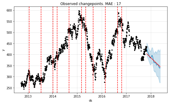
Eyeballing it we can see the points where trend has changed. You can also get the complete series of changepoints as a series. If the detected changepoints do not line up as you expect them to be, you can explicitly set them in the changepoints parameter.
model.changepoints.head()
40    2012-11-22
80    2013-01-21
120   2013-03-18
160   2013-05-20
201   2013-07-16
Name: ds, dtype: datetime64[ns]
This brings us to the end of this exploration of the fbProphet model. It would be a good idea to further read up on the inbuilt cross validation techniques that Prophet provides.

